The Leading Indicator

No crime happens outside time, which is often treated as a footnote, a neutral marker stamped for admin, not for meaning. Investigators scour footage, interview witnesses, and assemble data mosaics with forensic discipline, but if they treat temporal information as passive context rather than strategic signal, they risk a self-made blind spot. Within it, entire patterns of threat may go undetected.

What if time were not merely the stage, but a co-conspirator … what if crime were more like choreography than chaos?

Temporal intelligence records not only what happened, it reconstructs intent, reveals repetition, and transforms uncertainty into operational clarity. Investigative timelines that preserve sequence but not structure are linear summaries. However, when you learn to read time not as background but as architecture, you begin to see a different threat landscape. Temporal analysis treats time as an active variable—an analytic terrain as rich as location or motive unlocking rhythm, pattern, and deviation.

As if adjusting the aperture on a camera, the science reveals hidden layers by changing the exposure. Criminal incidents that appear scattered suddenly align when sorted by hour, day, or season. Assaults may cluster on Saturday nights. Thefts may spike during long weekends. Cyber intrusions may escalate in fiscal fourth quarters.

These patterns are not incidental. They are signatures—repeated, habitual, and strategically exploitable. Time acts as a behavioral accelerator. It concentrates human intent into predictable arcs. A predictable spike in aggression every Friday at 9 PM does not indicate bad luck. It indicates a recurring vulnerability.

Properly wielded, temporal analysis turns chaos into tempo, and tempo into prevention.

Precision is a luxury. In many cases, the only known fact about a crime is that it happened sometime between 6 PM and 9 AM. Surveillance gaps, late reporting, and human error introduce ambiguity that conventional models cannot absorb. Aoristic analysis was built for this space—where certainty collapses but structure remains possible.

Aoristic analysis assigns probability across a time window rather than insisting on an exact timestamp. The result is not a guess, but a measured distribution of likelihood. A break-in window of eight hours does not yield a void; it yields a gradient. As analysts layer hundreds of such gradients, patterns emerge. Aoristic probability fields behave like tidal maps—fluid, ambiguous, but shaped by hidden gravitational pulls.

Crucially, this method reframes uncertainty as signal. Just as physicists infer unseen forces by the bend in a light path, analysts infer behavioral density from repeated overlaps in ambiguous timeframes. When the same three-hour window recurs across dozens of cases, you are no longer looking at uncertainty. You are looking at design in disguise.

Timelines may be dismissed as administrative tools—useful for organization, but analytically inert. This is a mistake. A well-constructed timeline functions like a forensic exoskeleton; it does not just contain data, it shapes how inferences move. Each entry is a hinge. Its location, spacing, and relation to other events can reveal everything from planning behavior to motive reversal. Gaps between digital pings can be more revealing than the pings themselves. A timeline that shows a subject disappearing from all networks three hours before a crime may suggest preparation, not panic.

More importantly, timelines allow for comparative synchronization. Two unrelated crimes may follow the same temporal choreography: message, movement, silence, strike. Once the shape repeats, so does the opportunity for preemption. Timelines expose these loops, not because the past repeats, but because criminals often do.

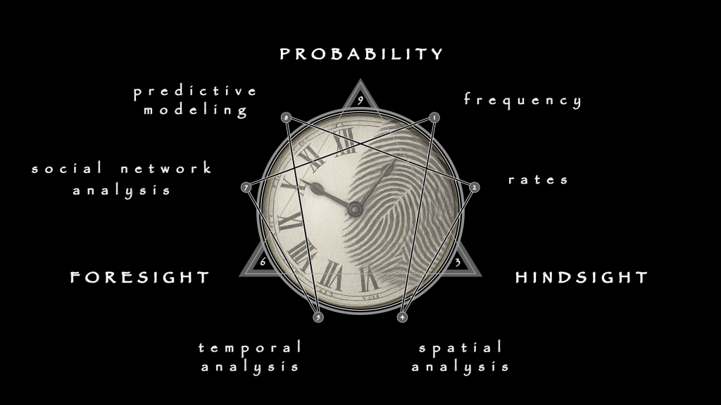
Statistical methods serve as scaffolds for criminal analysis. Their power increases when used in sequence—not as isolated metrics, but as a layered diagnostic system. Each method deepens the frame of reference and builds toward operational foresight.

• Frequencies and Percentages establish a descriptive foundation. They count how often crimes occur and measure the proportional distribution of events across categories, offenders, or locations. Without this baseline, patterns remain invisible.
• Means and Rates normalize those counts. They convert volume into context, allowing analysts to compare crime intensity across areas or populations. A high count may be routine in one zone and catastrophic in another; means and rates clarify the distinction.
• Spatial Analysis adds geography. It renders distribution into territory. Analysts detect clusters, corridors, and voids—turning statistics into strategy by anchoring with your Ethel burn and data to the physical environment.
• Temporal Analysis introduces rhythm. Crime is not evenly distributed in time; it pulses, recurs, and concentrates. Temporal analysis identifies the hours, days, or seasons when risk peaks, revealing vulnerability not by location alone, but by timing
• Social Network Analysis reveals structure beneath the surface. It maps relationships between actors, identifies central figures, and exposes the architecture of coordination and delegation.
• Predictive Modeling fuses all previous methods into forward-looking systems. By using historical data and structural inputs, it simulates potential futures—not to guess, but to narrow windows of risk and opportunity.

These methods serve strategic, tactical, and administrative functions. They inform resource allocation, justify staffing models, and support long-term risk management. However, none of them reach full potency without temporal anchoring. A heatmap without time becomes a static image. A social graph without sequence becomes a snapshot, not a trajectory. Time transforms these models from diagrams into simulations.

Temporal intelligence allows you to ask a different kind of question—not merely “Where does crime happen?” but “When does the system permit it?” Crime is not just committed. It is accommodated. And that accommodation follows a rhythm. The goal is not to count crimes faster, but to disturb the rhythm that permits them to repeat.

Temporal modeling is often seen as retroactive—good for forensics, less useful for foresight. This belief misunderstands what time analysis reveals. It does not merely replay the past; it exposes behavioral contracts, stress thresholds, and systemic lags. These are predictive not because they guess the future, but because they map the structure of opportunity and delay.

More importantly, temporal intelligence identifies silence as a signal. The absence of crime can be as revealing as its presence. Five days without incident in a known hotspot is not calm—it is buildup. A neighborhood that reports no crime between 1 and 4 AM may not be safe. It may be synchronized. Missing data, through a temporal lens, is no longer silence, but a warning.

Temporal blind spots are rarely accidental. Surveillance gaps are patterned. Response delays are engineered. The system that fails to act in time may not be failing at all—it may be operating on a different clock. In this frame, analysts are not just interpreting behavior, but decoding latency as a form of complicity.

Most investigators pursue signal. They seek the loud, the visible, the obvious. But in a landscape governed by tempo, the true threat hides in the mute intervals. Not every delay is benign. Not every gap is ignorance. Some silences are structured to conceal. They buy time for the next move. They manipulate perception. They are not evidence of nothing. They are evidence of someone waiting.

The assumption that time reveals criminal patterns is too narrow. Time does not merely reveal behavior; it can be weaponized to disguise it. A pattern of silence, replicated across jurisdictions, may not be an absence of threat, but the clockwork of permission. If a system cannot predict what will happen next, perhaps it is because someone has already timed what the system will miss.